Search

Mastering Dose-Response Curves: A Guide to Non-Linear Regression in GraphPad Prism

CLYTE research team
2 days ago
4 min read

Non-linear regression for dose-response curve in GraphPad Prism

Understanding how biological systems respond to varying doses of a drug, hormone, or toxin is fundamental in biomedical research. Dose-response curves provide crucial insights, but analyzing them effectively requires the right tools and techniques. Non-linear regression, particularly within software like GraphPad Prism, offers a powerful way to model these complex relationships, moving beyond simplistic linear assumptions to capture biological reality. This article summarizes key concepts and steps for performing non-linear regression for dose-response analysis in Prism, drawing from expert guides and resources.

You might also be interested in this IC50 vs EC50 article! Ask Sophie about your Non-Linear Regression data!

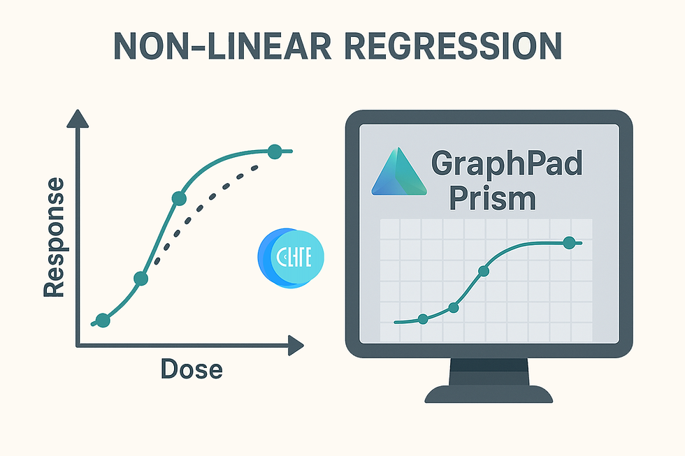
What is a Dose-Response Curve and Why Use Non-Linear Regression?

A dose-response curve plots the relationship between the dose (or concentration) of a substance (often plotted on a logarithmic scale) and the resulting biological effect. Many biological processes, like receptor binding governed by the law of mass action, inherently exhibit non-linear behavior. Plotting response against the logarithm of concentration typically yields a sigmoidal (S-shaped) curve.

While linear regression is simpler, attempting to linearize dose-response data (e.g., via Logit or Probit transforms, though not mentioned in detail in these specific sources) can distort experimental error and violate the assumptions of linear regression. Non-linear regression directly fits the data to a biologically relevant model without distorting transformations, providing more accurate parameter estimates. It's the preferred method for analyzing dose-response data.

Setting Up Your Data in GraphPad Prism

Data Preparation: Enter your data with the dose (or concentration) in the X column and the response in the Y column(s). If you have replicates, enter them in adjacent Y subcolumns.
X-Axis Transformation: Dose-response curves often span several orders of magnitude. It's standard practice to plot the X-axis on a logarithmic scale. You can either enter the logarithm of the concentrations directly into the X column or enter the concentrations and let Prism transform the axis.
Normalization (Optional): You might normalize responses to range from 0% to 100%. While this doesn't fundamentally change the fit, it can aid interpretation. Be cautious not to automatically exclude normalized values outside this range.
Avoid Smoothing: Do not smooth your data before fitting, as it distorts error and invalidates results like standard errors and confidence intervals.

Performing the Non-Linear Regression Analysis in Prism

Choose the Model: Prism offers built-in models. The most common for dose-response is the sigmoidal dose-response (variable slope) equation, also known as the four-parameter logistic (4PL) or Hill equation.

Y = Bottom + ( Top-Bottom ) / ( 1+10^( (LogEC50-X) * HillSlope))
Understand Parameters:
- Bottom: The minimum response plateau.
- Top: The maximum response plateau.
- LogEC50: The logarithm of the concentration that produces a response halfway between Top and Bottom. This is a key measure of potency. Fitting LogEC50 is preferred over fitting EC50 directly, as its uncertainty is more symmetrical on a log scale.
- HillSlope: Describes the steepness of the curve. A value of 1.0 is standard for simple binding; deviations suggest cooperativity or complex interactions.
Set Constraints: Crucially, decide if any parameters should be fixed (constrained) to constant values. If your data is normalized (e.g., 0% to 100%) or you have reliable controls defining the minimum or maximum response, constraining 'Bottom' and/or 'Top' can significantly improve the precision of the other parameters, especially LogEC50. However, only constrain if you are confident in the constant value. Data doesn't always define all parameters well (e.g., incomplete curves), making constraints necessary.
Initial Values: Prism usually generates good initial parameter estimates, but you can adjust them if needed.
Weighting: If scatter (variance) increases with the response level, consider relative weighting (weighting by 1/Y²). Otherwise, use the default (no weighting).
Global Fitting: If analyzing multiple related curves (e.g., with/without antagonist, different conditions), consider global non-linear regression. This fits all datasets simultaneously, sharing specified parameters (like Top, Bottom, or HillSlope) across curves while fitting others (like LogEC50) individually for each curve. This can greatly improve parameter precision, especially with incomplete curves.

Interpreting Your Results

Visual Check: Does the curve visually fit the data points well?
Parameter Plausibility: Are the best-fit values (Top, Bottom, LogEC50, HillSlope) scientifically reasonable? Is the EC50 within the range of tested concentrations?
Precision (Confidence Intervals): Examine the 95% confidence intervals (CI) for each parameter. Wide intervals indicate poorly determined parameters, possibly due to insufficient data range or scatter. The SE (Standard Error) helps calculate the CI.
Goodness-of-Fit (R²): R-squared (coefficient of determination) indicates the fraction of variance explained by the model. A high R² suggests the curve is close to the points, but doesn't guarantee the model is correct or parameters are well-defined.
Systematic Deviation: Check for runs test results or inspect a residuals plot. Non-random patterns suggest the chosen model may not be appropriate.
Model Comparison: If unsure between models (e.g., one-site vs. two-site, variable vs. fixed slope), Prism can compare them using statistical tests like the extra sum-of-squares F test or Akaike's Information Criterion (AIC). Only compare models if both yield sensible fits.

Common Pitfalls and Troubleshooting

Ambiguous Fits/Poorly Defined Parameters: Often occurs if data don't define the plateaus. Constraining Top/Bottom can help. Wide confidence intervals are a key indicator.
Model Too Complex: Fitting a two-site model when a one-site model suffices can lead to unreliable parameters with very wide confidence intervals. Use model comparison tests.
Bad Initial Values: Can cause the fit to fail ("Does not converge"). Check the curve generated by initial values.
Redundant Parameters: Sometimes a model is structured such that the data cannot distinguish between two parameters (e.g., determining k_on and k_off from a single association curve). This requires model reformulation or additional experimental data.

Conclusion

Non-linear regression in GraphPad Prism provides a robust framework for analyzing dose-response curves in biomedical research. By choosing appropriate models, setting sensible constraints, leveraging global fitting when applicable, and carefully interpreting the results, researchers can extract meaningful parameters like EC50 and HillSlope, quantifying potency and understanding the dynamics of biological responses. Remember to always combine statistical output with visual inspection and scientific judgment.

Wanna read more article like this!